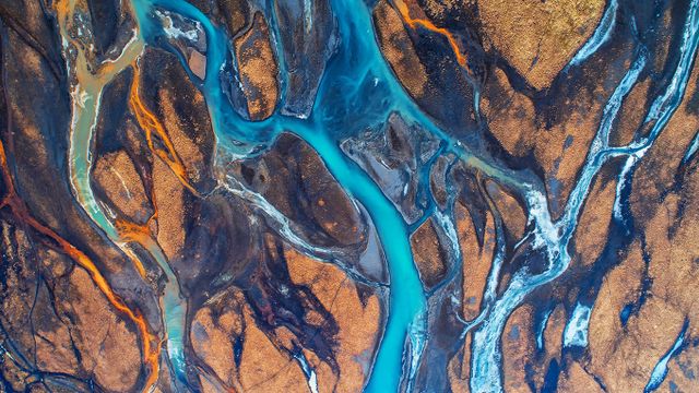
Applied Geospatial Analysis

Reach out to the team with any questions at commercial@bezerocarbon.com   

Transcript (edited for clarity)

Dr Phil Platts, Director of Geospatial & Earth Observation

I’d like to talk to you about our approach to geospatial analysis at BeZero Carbon, and how this applies to our assessment of risk in the Voluntary Carbon Market.

In short, our geospatial analysis provides a toolkit for assessing carbon projects anywhere in the world. We analyse carbon stocks and flows, inside and outside the project area, before, during and after project activities. This work informs the ratings process, and is accessible as interactive charts and maps on the BeZero Carbon Markets platform

In this presentation, I’ll first introduce our overall approach, including our team and the kinds of data we use, and then I’ll talk through some of the insights that we provide to ratings and clients.

Our approach at BeZero is a hybrid of quantitative, data and model-driven analysis, including machine learning and statistical modelling, combined with our expert judgement both in how the data are sourced and models constructed, and in the interpretation of outputs.

Every project is different, and every dataset or model has its uncertainties and limitations. Therefore, how we weigh these inputs in terms of credit risk, has to be highly nuanced, and under continuous review as the science advances, new information comes in, or as the situation evolves on the ground.

Our scientists have backgrounds at space agencies such as NASA, NGOs like the World Resources Institute, leading commercial entities such as tomtom and QuantumBlack (McKinsey), and academic institutions like Cambridge, Oxford and University College London.

Together we have extensive experience measuring carbon and biodiversity in the field, working with local communities and institutions, and strong track records in remote sensing and data science. In the geospatial team, we have published over 200 academic papers, which have been cited well over 10 thousand times.

Here’s an overview of some of the sources of Earth observation data that inform our analysis. The graphic is arranged to show the vertical distribution of remote sensing data at the top, down to in situ ground measurements at the bottom.

From space agencies we obtain data with typically global coverage at medium to coarse resolution, sometimes with long time series. 

From commercial partners we obtain higher resolution imagery, which is especially useful for monitoring low canopy density, planting and degradation. 

Closer to the surface, we make use of airborne LiDAR surveys. These are dense point clouds measuring the structure of vegetation - useful for estimating canopy height, cover and biomass. 

And then in situ ground measurements, of vegetation composition and structure, soil carbon, and biodiversity. These data are vital for understanding uncertainties in the remotely sensed data.

This is not an exhaustive list of our data sources. For example, we also use spatial data on land ownership, population densities, road networks, climate and so on.

In terms of outputs, our work informs the risk factors that we assess for carbon ratings. We provide overviews and insights through blogs and webinars, and journal articles. And we are building out our platform to surface more maps and charts to our users.

So, what exactly are we analysing here? What are the insights for assessing risk in the carbon markets?

We are broadly concerned with these three questions:

• To what extent are the carbon project’s activities common practice in the wider landscape?

• How accurately do we think emissions avoidance or removals have been quantified?

• And what is the risk that some or all of project impacts could be reversed or have already been reversed?
  

Firstly on common practice, the examples shown here are for a group of community-base tree planting projects in Kenya. We’re mapping all relevant carbon projects in the landscape - those are the colourful polygons clustered largely around Mount Kenya. For any projects where boundaries are not available on the registries, we digitise these manually in-house using imagery from documents.

In the upper map, the light blue speckles show gains in tree cover that has been achieved independently of carbon finance, so outside those project sites. In this case, the tree gain is quite minimal, and the particular project activity - supporting small scale landowners to plant mostly native trees - is especially uncommon.

In the lower panel, we’re mapping canopy height across the same landscape. This shows that most of the landscape is not forested, except for some old growth plantations and government forest reserves.

Now on carbon accounting, this can be simplified to the equation shown here, either by pixel or by forest strata:

ΔCO₂e  =  C  ×  (Baseline  –  Observed  –  Leakage)

Emissions avoided or removed is a function of four components.

The first is an estimate of the carbon stock density C - how much carbon is stored per unit area of land. This is typically used to scale area-based estimates of the net difference that a project is making.

The net difference is the baseline (without project scenario) minus what is observed in the project case, both inside the project area and outside the project boundaries due to leakage.

Our analysis interrogates each of these components of the emissions calculation, informing our view of additionality, over-crediting, and leakage.

Looking first at carbon stocks, it’s important to recognise that there is no perfect carbon map. There are numerous satellite-derived estimates, but none are accurate everywhere, and for any given location, the magnitude of the errors is generally unknown.

At BeZero, our approach is to use multiple carbon maps, derived using spaceborne and airborne LiDAR, radar and multispectral imagery. These are from governments, space agencies, academic labs and industry partners.

We validate these maps in-house in the project context, using a large database of ground-measured carbon. This database currently spans over 5,000 sites globally, and we are working with our partners to expand this further.

Through this combination of satellite remote sensing, extensive ground truth, and international collaboration, we are able to assess risk in project-reported carbon stocks anywhere in the world.

The next component we look at is the project’s assumed baseline.

Baselines are a counterfactual of what would have happened in the absence of a project. So for afforestation projects, the baseline is often zero - no trees planted, none lost. While for avoidance projects like REDD, the baseline is always above zero, indicating the amount of forest that would have been lost without project intervention.

These hypotheticals can never be directly observed. At BeZero we use statistically-matched, dynamic baselines to assess risk. This is similar in principle to the control group in clinical drug trials - the carbon finance is the treatment, and the controls are pixels in the surrounding region that are most similar to the project area (but which themselves are not subject to carbon finance).

Emissions in the project area and in matched controls are tracked over time, helping to isolate the impact of carbon finance.

Here’s a more in depth look at the matching process and its outcomes. The map at the top shows a project area in yellow. The aim is to find the most appropriate pixels to act as control sites in the surrounding landscape.

The first step is to set some limits on distance. We typically set a maximum distance of between 50 and 100-km from the project, while excluding a ring of land closest to the project, to avoid confounding effects of any leakage that might be occurring.

We then exclude any land parcels that have fundamentally different land ownership or protection status to the project, and also any other carbon projects that may be operating nearby.

This leaves us with the purple shaded region on the map. This can get quite complex, and require multiple stratifications, as different parts of the project may overlap with different combinations of land designation.

The second step is to select the most appropriate pixels from within this purple region. There is never a perfect set of matches, however, and so the process is bootstrapped - repeated many times to assess uncertainty.

The result of this second step is shown as the blue heat map - the more likely a pixel is to be a good match to the project, the deeper the shade of blue. In this second step, we are controlling for things like distance to past deforestation events, population pressure, accessibility by road or river, suitability for agriculture, and so on - as relevant to the particular project that we’re analysing.

The relative importance of these factors is quantified using a machine learning model, trained on historical patterns of forest loss in the wider region, and this helps guide what is included in the matching step.

In the example shown, we see that the project’s assumed baseline - plotted as the black line in the chart - is much higher than BeZero’s dynamic baseline would suggest is reasonable. This could indicate substantial risk of over-crediting.

The yellow line here plots actual forest loss inside the project area. For early vintages, this is actually higher than in the matched controls, indicating that the project - which permits logging - may have been emitting more carbon than it’s been avoiding.

For later vintages, the project is increasingly effective at avoiding deforestation, but still the baseline is probably too high.

Our scientists have been working on this for many months (and for years before that in their previous careers in conservation and disease risk mapping). We look forward to putting the results onto our platform later in the year.

An important component of the baselines work, and of monitoring more generally, is accurate detection of changes in the vegetation in and around project sites.

We use a range of products to facilitate this - including datasets from the University of Maryland, NASA, ESA, JAXA and industry partners.

Where we deem the accuracy of those datasets to be insufficient at the project level, we build segmentation models in-house, trained and validated locally to the project.

Two examples are shown here. On the left is an example of our forest segmentation model, built using data from space-borne LiDAR and 10-m Sentinel-2 satellite imagery.

While global models tend to misclassify forest cover in this landscape, and do not distinguish natural forests from the rubber plantations that replace them, our in-house model has much higher accuracy.

On the right is an illustration of some of the work we are doing to capture forest change in highly seasonal, open canopy systems such as those prevalent in eastern and southern Africa.

Here, we use deep learning to segment individual tree crowns. These are then used as training and validation data in models of canopy cover percentage and ultimately estimates of forest change.

The third key risk for carbon credits is non-permanence. That is, the risk that carbon emissions avoided or removed could be reversed in the future.

Here we look at fire risk using data from NASA, for example, and we are working with scientists and meteorologists on an ESA funded project to advance understanding of how fires spread and the impact on the carbon cycle.

We also construct drought models in house, to track historical conditions and to forecast future risk. This work combines climate data from the ECMWF, with soils data from ISRIC, and future climate projections from the IPCC.

The climate projections are also used to construct future scenarios of sea-level rise, particularly for mangrove projects.

And we assess the spatial distribution of common pests and diseases, which can be a risk especially for large single-species forest stands, common in the Improved Forest Management and Afforestation, Reforestation & Restoration sub-sectors.

Some reversal events are not in the future of course, but may have already occurred. We therefore monitor satellite data for evidence of material changes in the trend or extent of forest loss, prior to this being reported by projects or Standards Bodies.

The example here is of an avoided unplanned deforestation project in Brazil. While previously successful in protecting the project area from encroachment, we have detected a significant deforestation event that began after the date of last credit issuance.

By the end of 2022 this had become large enough to exceed the project’s buffer pool contribution, and we placed the project on watch. Following a review of all the evidence, we downgraded the project rating, while maintaining the watch status. We continue to monitor the extent of forest clearance, and await publication of documentation from the project referencing this loss event.

Dr Peter Wooldridge, Soil Carbon Lead

The following slides show some simplified examples of the extent to which geospatial analysis impacts ratings in different contexts.

In the first example, geospatial is paramount and largely determines the overall ratings.

In the second example, implications from GEO and non-GEO sources are much more balanced.

In the third example, evidence from GEO is largely outweighed by other factors

VCS 1689 looks to avoid deforestation of 67,791 ha of land on the edge of the recently declared Prey Long Wildlife Sanctuary.

The main drivers of deforestation in this system are those from small scale conversion to farming by local communities.

The baseline deforestation rates in the project area was set at 2.4% per year. Our analysis of deforestation rates since the project start date is closer to an annual average of 6% per year between 2015 and 2019.

This indicates that if the observed deforestation rate continues, forest area could be fully cleared in approximately 10 years from 2022. Therefore, no issued credits of any vintage would outlast the 30-year crediting period (2015-2045).

This analysis depicts significant over-crediting and non-permanence risks, as well as highlighting the limited effectiveness of the project at avoiding or preventing deforestation.

VCS 674 looks to avoid the conversion of over 47,000 ha of lowland tropical peat swamp ecosystem in Central Kalimantan, Indonesia.

The project’s reference regions were 11 concessions within a 100 km radius of the project area that have been, or are owned by the same agent of deforestation as the project.

Studies found that once a palm oil licence was obtained, conversion had occurred for 74.1% of the area in the first two years, and fully built out by year 6.

Rimba raya uses a minimum rate of conversion observed across any of the concessions in its reference region (calculated at 2,800 ha per year). It also applies a linear conversion rate and delays the development of two of its concessions for two years. The combination of these factors means the project possesses a highly conservative baseline. 

Through using BeZero’s Earth observation, we are able to validate the baseline it uses and therefore, its conservativeness.

Rimba Raya has experienced fire events throughout the project, which have caused forest loss events. Through using Earth observations, we can monitor the project area for fire and any associated burned area.

Fires across Indonesia are largely resultant of human activity and are closely linked to El Niño events, when prolonged drought occurs across the country.

Rimba Raya follows this national trend, with fires occurring during the strong El Niño event of 2015-2016, and the weak-moderate event of 2019.

Whilst carbon losses from fire events have been accounted for by the project, peatlands are typically low fire systems, so the re-occurrence of fires drives notable risks.

VCS2401 seeks to establish plantations on approximately 12,000 ha of land in Sierra Leone.

We find several positives in this project, such as that plantation forestry is not common practice in Sierra Leone, and accurately accounts for carbon stocks.

However, we find it unlikely that carbon finance was required to conduct project activities. There is no evidence for the consideration of carbon finance until after a large majority of the planting was undertaken, with planting occurring in 2014 and the project seeking carbon finance in 2019.

This also shows how the project shifted from not pursuing carbon finance originally, to subsequently pursuing it.

Moreover, we find the project received large quantities of external funding for conducting its plantation activities, potentially reducing its reliance on carbon finance.

These factors led to an overall low rating of project additionality. The rating is further constrained by a lack of evidence that the project attained its buffer pool contributions, based on credit issuance data.

George Carruthers, Senior Product Manager

We have made geospatial available on BeZero Carbon Markets through a dedicated tab on the project page for Nature Based Solutions (NBS) projects. Navigating to any NBS project, you will see a tab marked geospatial. Clicking on this brings up the map with a project area and other relevant boundaries loaded for the user to understand where in the world the project is.

We believe that we have one of the largest audited boundary sets in the Voluntary Carbon Market (VCM), with over 100 boundaries available to customers on the platform.

What sets BeZero data apart is how little boundary information is digitally available in the VCM. Only 55% of projects make a project area digitally available, and this is much less when considering REDD and REDD+ projects, and Reference Regions and Leakage Belts.

BeZero have painstakingly reconstructed and audited the boundaries of all projects in our NBS portfolio, and we have made this available to our clients.

Overlaid on these boundaries are data layers that we think will really benefit our clients. The way we have laid out our platform allows users to expand the layers of data we want to show users in the future, with the toggling feature giving them control of which data they want to analyse.

We have started with a partnership with the Integrated Biodiversity Assessment Tool, IBAT. With thousands of plotted areas, IBAT is the most comprehensive protected and key biodiversity area dataset in the world. 

The benefit to the user is being able to see how a project area and protected area interact, which gives them an indication of the additionality of a project.

Next, we will be expanding this over the coming months to visualise natural and human risks on the platform such as forest cover change and burned area maps, which has been a request of our customers.

Combining these data layers with the comprehensive BeZero boundary data set, we think this will form the basis for a powerful visual proposition and set up BeZero for success in the market when it comes to geospatial capability.

Being able to see the topography of a landscape is also important for our users, where decisions are influenced by the altitude of a project. 

The example shown here, VCS 612, clearly shows how the project area is defined partly based on elevation. With the satellite map also turned on, you can also see how the vegetation type changes with elevation and provides an understanding of how the project boundary was chosen.